Type @rating to add a smart chip in Google Sheets on the web for a viewer-friendly way to display zero-to-five star scores.
Google Sheets lets you enter star ratings in cells with a smart chip. Since many people find stars easier to differentiate at a glance than a list of numbers, this feature may be useful wherever you want to rate products, features, media, apps, places or services. The feature offers the same sort of 5-star format used in Android and Apple app stores and at Amazon, Uber and Yelp.
You may format cells for star ratings in Google Sheets on the web. Once formatted, you may select and enter a rating either in Google Sheets on the web or in the Google Sheets mobile apps on Apple or Android devices.
Jump to:
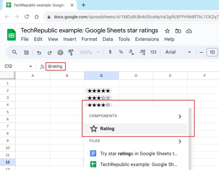
Working with stars in a Google Sheet is a two-part process. First, you configure a cell to show stars, and then you or your collaborators can enter a star rating. To format a cell for ratings:
Figure A
Once a cell has been formatted to display a star rating, you may enter the rating either on the web or in Google Sheets on a mobile device.
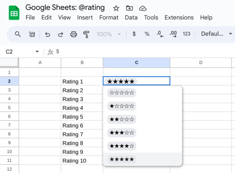
To enter stars while in a web browser, such as Google Chrome:
Figure B

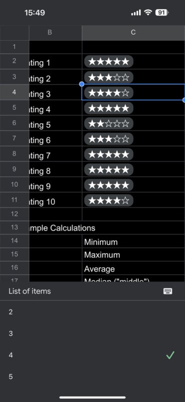
To enter stars in the Google Sheets mobile app on Android, iPhone or iPad:
Figure C

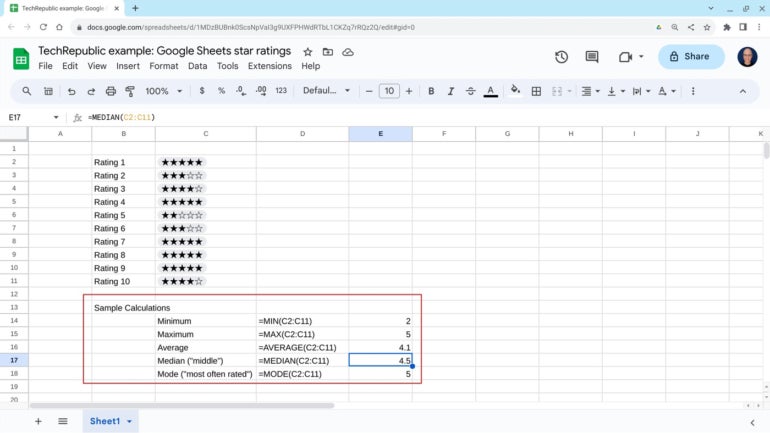
Ratings in Google Sheets are reflected as the numbers zero to five, which means you may obtain values from each star rating cell. The following formulas can help you evaluate a range of star ratings in Google Sheets (Figure D).
Figure D

The Min and Max formulas return the lowest and highest numbers from a set, respectively. For example:
=Min(C2:C11)
=Max(C2:C11)
The difference between the Min and Max indicates the full range of people’s ratings. For example, a Min of 3 and a Max of 4 indicates agreement on a mid-range score from responders, compared to a Min of 1 and a Max of 5, which signals a wider range of ratings.
The average of a set of stars will be somewhere between 0 and 5, and can indicate the overall consensus across all ratings. When comparing two ratings, the higher average generally reflects overall higher ratings. To calculate the average, the system adds all ratings, then divides the total by the number of ratings received. For example:
=Average(C2:C11)
The median is the value that separates a set in half, with half of the ratings above the median and half of the ratings below it. In contrast to the average, which can be affected by a few extremely high or low ratings, you might think of the median as reliably reflecting the middle of a set. To obtain the median, use a formula such as:
=Median(C1:C11)
Mode returns the rating most frequently found in a set. For example, in a set of 10 ratings, if four of those are two stars, three are four stars, and three are five stars, the mode would be two stars. For example:
=Mode(C2:C11)
Unlike the above formulas, which will always return a result, Mode might not. For example, in a set of 10 ratings, if two people each rated items one, two, three, four and five stars, there would be no mode. Since each of the possible ratings would have received two results, there would be no single rating that received the most. Similarly, if star ratings are split between two numbers (e.g., five people rated an item as four stars, and five people rated it as five stars), again, there would be no mode.
Mention or message me on Mastodon (@awolber) to let me know how you use star ratings and related calculations in Google Sheets.